Movie Box Office Revenue Prediction
The movie box office revenue prediction is a problem that is widely being worked on by researchers and production houses. In our problem, the revenue prediction has been designed as a multinomial classification problem with 10 revenue buckets - the lowest revenue bucket implying a flop and the highest revenue bucket implying a blockbuster.
The raw movie dataset sourced from Kaggle had entries for 4803 movies. In addition to our target variable revenue, the dataset had a range of features including information around budget, cast, crew, movie genre, movie synopsis, production company etc. These features had to be engineered to suitable numeric/categorical features prior to modelling. In our final modelling data, after exploring a range of features we fed 71 features into the models.
The 3 primary statistical modelling techniques that were used to solve this multinomial classification problem were Elastic Net, Random Forest and XGBoost. The three models were then used to create a rule-based ensemble model. The techniques were compared using manual K-fold cross validation. Random Forest showed the best performance measure among the primary modeling techniques.
The 2 performance metrics used to evaluate models through K-Fold Cross Validation were :
- Average percentage of classifying a movie performance in the exact class - Bingo Classification Accuracy
- Average percentage of classifying a movie performance within one class of its true performance - 1 Away Classification Accuracy
1 Motivation
The global box office revenue is projected to scale 50bn USD by 2020. The fact that movie making is an expensive business, makes it extremely imperative to ensure that movies experience box office success. Knowing which movies are likely to fail/succeed prior to the movie release is the holy grail for movie makers. Movie box office revenue prediction prior to movie release can help production companies save millions of dollars. The scope to perform innovative feature engineering and a large interest this problem has gained among scholars was our primary motivation behind picking this problem.
2 Literature Review
There has been a quite a lot of work around the movie box office revenue prediction problem. One of the most cited work for this specific problem is the paper “Predicting box-office success of motion pictures with neural networks”, and the author is Ramesh Sharda. He used neural networks as the main algorithm to perform box office prediction on a subset of our data. We referred to prior literature and adopted identical problem formulation(as a multinomial classification), model evaluation metrics to enable better benchmarking of our results.
3 Data Preparation
Our base data consists of two csv files containing information about 5000 movies and the list of their cast and crew members ( in the same order as they appear in the movie credits) downloaded from Kaggle (https://www.kaggle.com/tmdb/tmdb-movie-metadata/data). The original schemas of these two datasets are as follows,
Movie File Schema:
names(movies)
##  [1] "ï..budget"            "genres"               "homepage"
##  [4] "id"                   "keywords"             "original_language"
##  [7] "original_title"       "overview"             "popularity"
## [10] "production_companies" "production_countries" "release_date"
## [13] "revenue"              "runtime"              "spoken_languages"
## [16] "status"               "tagline"              "title"
## [19] "vote_average"         "vote_count"
Credits File Schema:
names(credits)
## [1] "movie_id" "title" "cast" "crew"
The data preparation process involved four main steps:
3.1 Data Cleaning
Some rows of data had a lot of missing values and some others were improperly formatted. In this step, we filtered cleaned or removed such rows to ensure the data is clean and ready to use.
3.2 Data Parsing
Since a lot of the data in columns was stored as JSON arrays, we had to manipulate the dataframe to extract relevant information from these columns. We extracted the first 2 genres, first 2 production houses, first 2 keywords, first 6 cast members and crew members in important positions like Producer, Director etc. We did this on the entire dataset. We have shown a sample code for parsing the genres column below. The other JSON columns were parsed similarly and stored in csv files.
library(jsonlite)
library(dplyr)
movies.cleaned = movies
cols <- names(movies.cleaned)
numbers <- seq(1,2)
for(n in numbers)
{
genre_id_col = paste0("genre_id_",n)
genre_col = paste0("genre_",n)
movies.cleaned[[genre_id_col]] <- apply(movies,1,function(x)
{
  res=fromJSON(x[2])
  val <- ifelse(is.data.frame(res),
                 {
                   res <- res %>%
                     mutate_all(as.character)
                   ifelse(is.null(res$id[n]),"",res$id[n])
                 },"")
  val
})
movies.cleaned[[genre_col]] <- apply(movies,1,function(x)
{
  res=fromJSON(x[2])
  val <- ifelse(is.data.frame(res),
                {
                  res <- res %>%
                    mutate_all(as.character)
                  ifelse(is.null(res$name[n]),"",res$name[n])
                },"")
  val
})
}
movies.cleaned$genre_num <- apply(movies,1,function(x)
{
  res=fromJSON(x[2])
  ifelse(is.data.frame(res),nrow(res),0)
})
movies.cleaned <- movies.cleaned[ , !(names(movies.cleaned) %in% c("genres"))]
3.3 Data Enrichment
For cast and crew members in the original data, we sourced popularity, birthdates and overview from TMDB using the TMDB API. Thus, we enriched the original dataset with popularity indicator, age, and mentions of academy award or golden globe in their overview(assuming these will only be mentioned if the person is nominated or wins the respective awards) of the cast and crew members. We have retrieved this information using the API and stored it in csv files for enriching our existing dataset. The csv files are then imported and integrated with the existing dataset for data enrichment as shown in the snippet below.
#Example tmdb API code
#info = person_tmdb("dc0c751ee576a078b7dc68b7f9ffa1b6",crew_id)

#read the info pulled from TMDB stored in csv files
cast_info <- read.csv("clean_cast_info.csv")
crew_info <- read.csv("clean_crew_info.csv")
credits.cleaned <- merge(credits.cleaned,cast_info,by="movie_id")
credits.cleaned <- merge(credits.cleaned,crew_info,by="movie_id")
movies.cleaned <- merge(movies.cleaned,credits.cleaned,by.x="id",by.y="movie_id")
castnums <- seq(1,6)
bdaycols <- c()
agecols <- c()
for(castnum in castnums)
{
  agecol <- paste0("castage_",castnum)
  agecols  <- c(agecols,agecol)
  bdaycol <- paste0("birthday_00",castnum)
  bdaycols <- c(bdaycols,bdaycol)
  movies.cleaned[[agecol]]<- as.integer(as.Date(movies.cleaned$release_date,"%d/%m/%y")-as.Date(movies.cleaned[[bdaycol]]))/365.25
}
movies.cleaned <- movies.cleaned[ , !(names(credits.cleaned) %in% bdaycols)]
3.4 Data Filtering and Imputation
We noticed missing/suspicious data especially in the budget and revenue columns which are two of the most important columns for our model. We used a cutoff of 10,000$ on revenue as exclusion criteria and excluded any rows with revenue less than that for the purpose of our actual model. This threshold was set to remove films with incomplete revenues reported. We also included only English Films to ensure that the movies had movie box office revenues reported in US Dollars. For movies with missing budget information, we manually researched online and entered the budget.
4 Feature Creation
Some interesting features that we believed would be valuable for the model were created in the feature engineering stage. Examples of features we created include :
- Historical Performances of Crew and Cast in terms of Revenue, IMDB Ratings
- Network Interaction Effect between Crew and Cast
- Prior Academy Award Nominations of the Cast and Crew
- Historical Collection of Production Company making the movie
- Time features around movie release
- Competition during movie release
4.1 Social Network of Movies
Apart from these we decided to create some social network based features to analyze the network effect of the people and production houses involved with a movie. e.g. One hypothesis is that the movie performance could be higher if the producer of the movie:
i) Has made more movies and highly rated movies earlier
ii) Has worked with diverse genres earlier
iii) Has made more movies and highly rated movies of this particular genre earlier
iv) Has made more movies with other production houses/actors who are strong players in the industry
Such hypothesis applies to directors, top cast members as well as production companies.
To capture this network effect, we have created a social network of movies, producers, directors, top cast members and production companies. Every movie, producer, director, actor, production company is represented as a node. We have an edge between a movie and a producer/director/actor/production company if they were involved in this particular movie. The weight of this edge is given by the voter’s rating for the movie in TMDB, i.e highly rated movies have heavier edges. We have then calculated the eigenvector centrality of each node to calculate the strength of network effect for that node. While calculating this eigenvector centrality, we had to be careful that the metric calculated for a movie only takes into account the subnetwork consisting of movies released before this movie (Otherwise we will be encoding the future in our model) We have included a small example of how the computation for network interaction features was done below:
#Example social network code
#get nodes df - id, label, tmdb_id, type
#get crew members and create nodes for all of them
nodes.people = data.frame(id="",attr="",type="",stringsAsFactors = FALSE)
nodes.people <- nodes.people[1==0,]
for( j in jobs)
{
  crew.filter <- movies.demo[j]
  crew.filter <- unique(crew.filter)
  names(crew.filter) <- c("id")
  nodes.people.filter <- crew.filter
  nodes.people.filter$attr <- j
  nodes.people.filter$type = "person"
  nodes.people <- rbind(nodes.people,nodes.people.filter)
  rm(nodes.people.filter)
  rm(crew.filter)
}
nodes.people <- na.omit(nodes.people)
#get list of movies and create nodes for all of them
node.movies <- data.frame(id=movies.demo$id,attr=movies.demo$genre_1,stringsAsFactors=FALSE)
node.movies$type <- "movie"
node.movies <- na.omit(node.movies,cols="id")
#combine movie and people nodes into the complete node list
node.all <- rbind(nodes.people,node.movies)
node.all$label <- paste(node.all$type,node.all$id,sep =" ")
node.all$tmdb_id <- node.all$id
node.all$id <- node.all$label
node.all <- node.all[!duplicated(node.all[,c('id')]),]
#get edges df - source, target, type, id, weight, release date
#each edge has the following attributes: weight, release_date, genre, attr( this stores the relationship type like director/producer etc)
edges <- data.frame(source ="",target="",weight=0,release_date=date(),attr="",genre="",stringsAsFactors = FALSE)
edges <- edges[1==0,]
for(j in jobs)
{
movie.filter <- movies.demo[,c("id","vote_average", "release_date","genre_1",j)]
names(movie.filter) <- c("source","weight","release_date","genre","target")
movie.filter <- na.omit(movie.filter)
edges.filter <-movie.filter
edges.filter$target <- paste("person",edges.filter$target,sep=" ")
edges.filter$source <- paste("movie",edges.filter$source,sep=" ")
edges.filter$attr <- j
edges <- rbind(edges,edges.filter)
rm(movie.filter)
rm(edges.filter)
}
#create network
#create network
require("igraph")
movies.net <- graph_from_data_frame(d=edges.all, vertices=node.all, directed=F)
A sample network indicating the movie-director relationship can be viewed below,
require("igraph")
movies.net <- graph_from_data_frame(d=edges, vertices=node.all, directed=F)
deg <- degree(movies.net, mode="all")
V(movies.net)$size <- deg*8
colrs <- c("tomato", "gold")
V(movies.net)$color <- colrs[V(movies.net)$type]
V(movies.net)$color<-ifelse(V(movies.net)$type=="person","tomato","gold")
E(movies.net)$edge.color <- "gray80"
plot(movies.net, vertex.frame.color="#ffffff", edge.arrow.size=3)
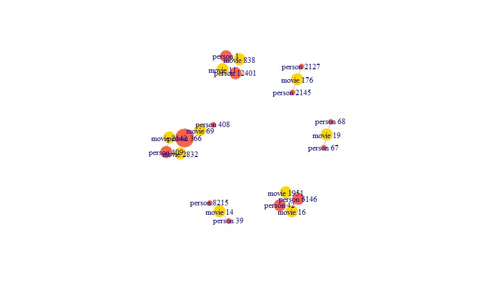
Using such relationship strengths between cast, crew and movies, Eigen scores were created and fed into the models to predict revenue. The features created in this manner were pre computed and stored to be imported for the final model.
4.2 Time Based Features
We also created some other features as follows:
-
Month of release
-
Days to nearest holiday around movie released
-
Number of movies released in a 2 week window around the movie release date (As a proxy for competition)
-
Consumer Price Index for month and year as a proxy for inflation
These features were primarily to account for the time differences of when the movies were released.
4.3 Historical Movie Features
When we looked at movies revenues and performance, we hypothesized that the performance of the movie has a strong relationship with how the crew, cast, production company of the movie have fared in the past. We decided to create a historical revenue, historical movie count and historical count of IMDB votes and rating for the primary cast, crew and production company associated with the movie.
We have shown a sample snippet below of how we created one of the mentioned features.
base<-read.csv("tmdb_5000_movies_final.csv",header=T,stringsAsFactors = F)
historial_sample<-merge(x=base,y=crew,by.x="id",by.y="movie_id",all.x=T)
####Aggregate Historical Revenue and # of Films for each Producer of a film###
historical_sample<-historical_sample[,c("id","revenue","release_date","Producer")]
historical_sample_order<-historical_sample[with(historical_sample,order(Producer,release_date)),]
historical_sample_order$csum <- ave(historical_sample_order$revenue, historical_sample_order$Producer, FUN=cumsum)
historical_sample_order$HistoricalRevenue_Producer<- historical_sample_order$csum - historical_sample_order$revenue
historical_sample_final <- historical_sample_order %>% group_by(Producer) %>% mutate(HistoricalNoofFilmsProducer=row_number()-1)
features_df<-historical_sample_final[,c("id","HistoricalRevenue_Producer","HistoricalNoofFilmsProducer")]
historical_data_integrated<-merge(movies.cleaned,features_df,by=c("id"))
The same procedure was repeated to compute historical features for other fields.
5. Modelling Overview
The problem is designed to be a multi class classification problem and we are trying to predict the revenue bucket a movie will fall into. Having explored a range of predictors in the feature creation section, 71 shortlisted features were fed into the models to predict the revenue bucket.
The revenue bucket cutoffs have been identified by breaking the continuous revenue variable into deciles. We have revenue buckets ranging from 1 (flop movie) to 10(blockbuster) into which we can classify the movie into. This method helps avoid class imbalance in the target variable.
In the snippet below, we pre load the final dataset named data_movies with all features in the working environment and then create the multi-class target variable as discussed.
require(dplyr)
##The model ready, integrated dataset data_movies has been pre loaded in the working environment###
data_movies$revenuebuckets<-ntile(data_movies$revenue,10)
data_movies$revenuebuckets<-as.factor(data_movies$revenuebuckets)
The revenue cutoffs for each of the 10 buckets can be seen below.
quantile(data_movies$revenue, prob = c(0, 0.10,0.20,0.30,0.40,0.50,0.60,0.70,0.80,0.90,1))
##         0%        10%        20%        30%        40%        50%
##      10000    4278786   12005656   22327409   36202281   55157539
##        60%        70%        80%        90%       100%
##   82423241  117817332  177281841  311290345 2787965087
To evaluate the model, we use manual K-Fold cross validation to compare the accuracy of our predictions. We have defined the K-folds of the dataset in the snippet below to ensure consistency while comparing models.
K <- 10
n <- nrow(data_movies)
set.seed(100)
shuffled.index <- sample(n, n, replace=FALSE)
data_movies[shuffled.index, "fold"] <- rep(1:K, length.out=n)
5.1 Elastic Net Model
The Elastic Net algorithm works by shrinking the beta coefficients of less important variables towards zero. It has two main parameters to tune - alpha and lambda. Lambda is the penalty coefficient and it’s allowed to take any number. Alpha refers to the type of model we want to try and ranges from 0 to 1. If alpha = 0, we have a ridge model and if alpha = 1, we have a LASSO model and any value in between is an intermediate elastic net. Since our problem is a multi-class classification problem, we have used the multinomial family in the elastic net to build our model.
We obtained an optimal alpha value of 1 and optimal 1SE lambda value of 0.006 as seen from the table below.
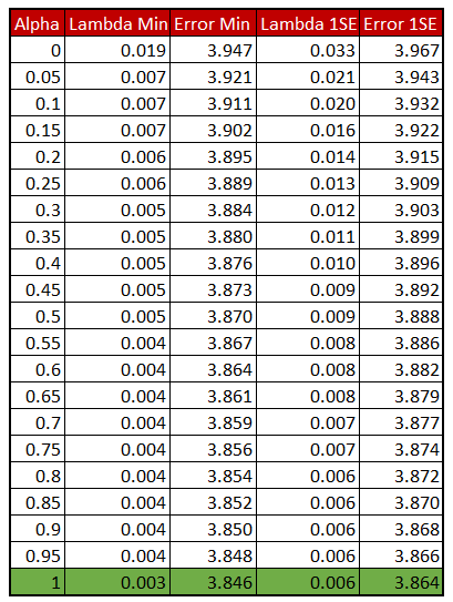
To compare the champion elastic net Model with other models we deploy manual K-Fold cross validation. We have already made 10 folds on our dataset and we will use them for getting our confusion matrix, bingo classification accuracy and 1-Away classification accuracy of the elastic net model.
en.lam=0.006040416
en.alpha=1
require(glmnet)
en.mod <- glmnet(x.elasticnet, y.elasticnet, alpha=en.alpha, family="multinomial")
######K Fold Cross Validation#######
K <- 10
data_movies$el.predict<- NA
# start the k-fold CV
require(glmnet)
for (k in 1:K) {
x.elasticnet.kfold <- model.matrix(revenuebuckets ~ HistoricalRevenue_Director+HistoricalNoofFilmsDirector+HistoricalRevenue_Producer+HistoricalNoofFilmsProducer+HistoricalRevenue_Composer+HistoricalNoofFilmsComposer+HistoricalRevenue_Writer+HistoricalNoofFilmsWriter+HistoricalRevenue_castid_001+HistoricalNoofFilmscastid_001+HistoricalRevenue_castid_002+HistoricalNoofFilmscastid_002+HistoricalRevenue_castid_003+HistoricalNoofFilmscastid_003+CrimeGenre+AdventureGenre+AnimationGenre+ComedyGenre+DramaGenre+ActionGenre+WesternGenre+ScienceFictionGenre+MysteryGenre+ThrillerGenre+RomanceGenre+FantasyGenre+HorrorGenre+WarGenre+FamilyGenre+DocumentaryGenre+MusicGenre+HistoryGenre+ForeignGenre+noofproductionhouses+HistoricalRevenue_PrimaryProductionHouse+ runtime+budget+inflationovertheyears+ competitionscore+monthofrelease+eigenscore_net+
eigenscore+releaseyear+HistoricalVoteCount_Actor+HistoricalVoteCount_PrimaryProductionHouse+HistoricalVotes_Director+HistoricalVotes_Producer+director_flexibility+producer_flexibility+eigenscore_bygenre_Director+eigenscore_full_Director+eigenscore_bygenre_Producer+eigenscore_full_Producer+eigenscore_bygenre_Screenplay+eigenscore_full_Screenplay+eigenscore_bygenre_Writer+eigenscore_full_Writer+eigenscore_bygenre_Composer+eigenscore_full_Composer+eigenscore_bygenre_cast+eigenscore_full_cast+eigenscore_bygenre_prodcomp_02+eigenscore_full_prodcomp_02+academynom_001+academynom_002+academynom_003+academynom_004+ggnom_001+ggnom_002+ggnom_003+ggnom_004,data=data_movies[data_movies$fold!=k,])[,-1]
y.elasticnet.kfold <- data_movies[data_movies$fold!=k,"revenuebuckets"]
el.fitted <- glmnet(x.elasticnet.kfold, y.elasticnet.kfold, alpha=en.alpha, family="multinomial")
x.elasticnet.kfold.test <- model.matrix(revenuebuckets ~ HistoricalRevenue_Director+HistoricalNoofFilmsDirector+HistoricalRevenue_Producer+HistoricalNoofFilmsProducer+HistoricalRevenue_Composer+HistoricalNoofFilmsComposer+HistoricalRevenue_Writer+HistoricalNoofFilmsWriter+HistoricalRevenue_castid_001+HistoricalNoofFilmscastid_001+HistoricalRevenue_castid_002+HistoricalNoofFilmscastid_002+HistoricalRevenue_castid_003+HistoricalNoofFilmscastid_003+CrimeGenre+AdventureGenre+AnimationGenre+ComedyGenre+DramaGenre+ActionGenre+WesternGenre+ScienceFictionGenre+MysteryGenre+ThrillerGenre+RomanceGenre+FantasyGenre+HorrorGenre+WarGenre+FamilyGenre+DocumentaryGenre+MusicGenre+HistoryGenre+ForeignGenre+noofproductionhouses+HistoricalRevenue_PrimaryProductionHouse+ runtime+budget+inflationovertheyears+ competitionscore+monthofrelease+eigenscore_net+
eigenscore+releaseyear+HistoricalVoteCount_Actor+HistoricalVoteCount_PrimaryProductionHouse+HistoricalVotes_Director+HistoricalVotes_Producer+director_flexibility+producer_flexibility+eigenscore_bygenre_Director+eigenscore_full_Director+eigenscore_bygenre_Producer+eigenscore_full_Producer+eigenscore_bygenre_Screenplay+eigenscore_full_Screenplay+eigenscore_bygenre_Writer+eigenscore_full_Writer+eigenscore_bygenre_Composer+eigenscore_full_Composer+eigenscore_bygenre_cast+eigenscore_full_cast+eigenscore_bygenre_prodcomp_02+eigenscore_full_prodcomp_02+academynom_001+academynom_002+academynom_003+academynom_004+ggnom_001+ggnom_002+ggnom_003+ggnom_004,data=data_movies[data_movies$fold==k,])[,-1]
data_movies[data_movies$fold == k, "el.predict"] <- as.numeric(predict(el.fitted, newx =x.elasticnet.kfold.test,s=en.lam,type="class"))
}
The 10*10 confusion matrix for the elastic net Model can be seen as follows,
###Confusion Matrix####
#table(data_movies$revenuebuckets, data_movies$el.predict)
cm_el<- as.matrix(table(Actual=data_movies$revenuebuckets,Predicted= data_movies$el.predict))
cm_el
##       Predicted
## Actual   1   2   3   4   5   6   7   8   9  10
##     1  250  35  10   7   5  11   1   2   0   0
##     2  140  77  31  20  10  12   9  10   9   2
##     3  106  55  38  29  16  26  13  19  14   5
##     4   75  50  54  28  19  28  23  17  20   6
##     5   59  39  51  27  16  39  31  35  17   7
##     6   45  19  38  30  23  29  40  47  35  14
##     7   25  27  30  13  30  43  42  40  47  24
##     8   11  19  12  15  19  39  34  49  79  43
##     9   12   9  12  10   5  13  28  52  98  82
##     10   2   5   9   7   2   6   9   8  47 225
cmdf_el<- as.data.frame(cm_el)
cm_rs_el<-reshape(cmdf_el,idvar="Actual",timevar="Predicted", direction="wide")
cm_rs_el$Actual<-NULL
rowsums = apply(cm_el, 1, sum)
cm_rs_el$TotalActuals<- rowsums
acc_fold_el<-c()
for (i in 1:nrow(cm_rs_el))
  acc_fold_el[i]<-cm_rs_el[i,i]/cm_rs_el[i,"TotalActuals"]
The bingo classification accuracy for the elastic net Model is as follows,
final_acc_el<- mean(acc_fold_el)
final_acc_el
## [1] 0.2658178
5.2 Random Forest Model
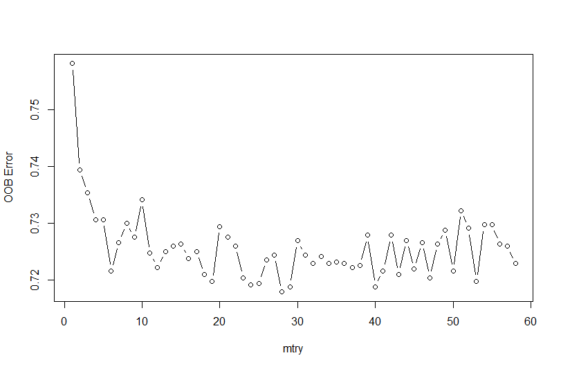
In the random forest model for multi-class classification, we have tuned the mtry parameter. Mtry parameter in random forest refers to the number of features we select by random sampling while building each tree in the forest. We have obtained an optimal mtry of 28 as seen from the following plot.
require(randomForest)
rf_overall <- randomForest( revenuebuckets~HistoricalRevenue_Director+HistoricalNoofFilmsDirector+HistoricalRevenue_Producer+HistoricalNoofFilmsProducer+HistoricalRevenue_Composer+HistoricalNoofFilmsComposer+HistoricalRevenue_Writer+HistoricalNoofFilmsWriter+HistoricalRevenue_castid_001+HistoricalNoofFilmscastid_001+HistoricalRevenue_castid_002+HistoricalNoofFilmscastid_002+HistoricalRevenue_castid_003+HistoricalNoofFilmscastid_003+CrimeGenre+AdventureGenre+AnimationGenre+ComedyGenre+DramaGenre+ActionGenre+WesternGenre+ScienceFictionGenre+MysteryGenre+ThrillerGenre+RomanceGenre+FantasyGenre+HorrorGenre+WarGenre+FamilyGenre+DocumentaryGenre+MusicGenre+HistoryGenre+ForeignGenre+noofproductionhouses+HistoricalRevenue_PrimaryProductionHouse+ runtime+budget+inflationovertheyears+ competitionscore+monthofrelease+eigenscore_net+
eigenscore+releaseyear+HistoricalVoteCount_Actor+HistoricalVoteCount_PrimaryProductionHouse+HistoricalVotes_Director+HistoricalVotes_Producer+director_flexibility+producer_flexibility+eigenscore_bygenre_Director+eigenscore_full_Director+eigenscore_bygenre_Producer+eigenscore_full_Producer+eigenscore_bygenre_Screenplay+eigenscore_full_Screenplay+eigenscore_bygenre_Writer+eigenscore_full_Writer+eigenscore_bygenre_Composer+eigenscore_full_Composer+eigenscore_bygenre_cast+eigenscore_full_cast+eigenscore_bygenre_prodcomp_02+eigenscore_full_prodcomp_02+academynom_001+academynom_002+academynom_003+academynom_004+ggnom_001+ggnom_002+ggnom_003+ggnom_004,data=data_movies,importance=TRUE,mtry=28)
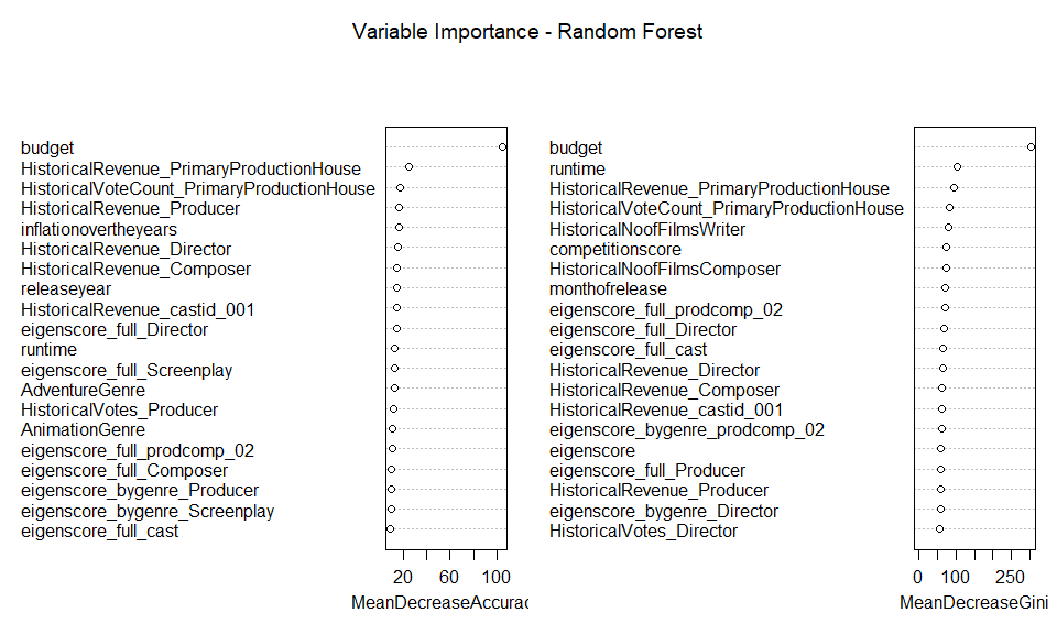
We can use the tuned mtry to build a model on the complete dataset to get the variable importance of the predictors. The variable importance of top 20 predictors are displayed below,
require(randomForest)
varImpPlot(rf_overall, main="Variable Importance - Random Forest", n.var=20)
To compare the champion random forest model with other models we deploy manual K-Fold cross validation. We have already made 10 folds on our dataset and we will use them for getting our evaluation metrics. The K-Folds used for cross validation are consistent with the ones used in the prior elastic net model.
data_movies$rf.predict<- NA
require(randomForest)
for (k in 1:K) {
  rf.fitted <- randomForest(revenuebuckets ~ HistoricalRevenue_Director+HistoricalNoofFilmsDirector+HistoricalRevenue_Producer+HistoricalNoofFilmsProducer+HistoricalRevenue_Composer+HistoricalNoofFilmsComposer+HistoricalRevenue_Writer+HistoricalNoofFilmsWriter+HistoricalRevenue_castid_001+HistoricalNoofFilmscastid_001+HistoricalRevenue_castid_002+HistoricalNoofFilmscastid_002+HistoricalRevenue_castid_003+HistoricalNoofFilmscastid_003+CrimeGenre+AdventureGenre+AnimationGenre+ComedyGenre+DramaGenre+ActionGenre+WesternGenre+ScienceFictionGenre+MysteryGenre+ThrillerGenre+RomanceGenre+FantasyGenre+HorrorGenre+WarGenre+FamilyGenre+DocumentaryGenre+MusicGenre+HistoryGenre+ForeignGenre+noofproductionhouses+HistoricalRevenue_PrimaryProductionHouse+ runtime+budget+inflationovertheyears+ competitionscore+monthofrelease+eigenscore_net+
eigenscore+releaseyear+HistoricalVoteCount_Actor+HistoricalVoteCount_PrimaryProductionHouse+HistoricalVotes_Director+HistoricalVotes_Producer+director_flexibility+producer_flexibility+eigenscore_bygenre_Director+eigenscore_full_Director+eigenscore_bygenre_Producer+eigenscore_full_Producer+eigenscore_bygenre_Screenplay+eigenscore_full_Screenplay+eigenscore_bygenre_Writer+eigenscore_full_Writer+eigenscore_bygenre_Composer+eigenscore_full_Composer+eigenscore_bygenre_cast+eigenscore_full_cast+eigenscore_bygenre_prodcomp_02+eigenscore_full_prodcomp_02+academynom_001+academynom_002+academynom_003+academynom_004+ggnom_001+ggnom_002+ggnom_003+ggnom_004 ,data=data_movies,subset=(fold != k),mtry=28)
data_movies[data_movies$fold == k, "rf.predict"] <- predict(rf.fitted, newdata=data_movies[data_movies$fold == k, ],type="response")

}
The 10*10 confusion matrix for the random forest model on manual K-Fold cross validation can be seen below,
####Confusion matrix Creation###
cm_rf<- as.matrix(table(Actual=data_movies$revenuebuckets,Predicted= data_movies$rf.predict))
cm_rf
##       Predicted
## Actual   1   2   3   4   5   6   7   8   9  10
##     1  199  51  26  17  15   7   2   2   2   0
##     2   85  79  44  32  30  20  10   9   9   2
##     3   52  49  59  47  35  30  16  13  18   2
##     4   30  37  58  42  43  41  25  33   8   3
##     5   28  22  38  47  40  47  35  40  16   8
##     6   14  20  29  29  41  53  51  50  19  14
##     7   10  10  23  30  28  47  43  72  40  18
##     8    2   6  18  18  27  25  60  66  71  27
##     9    6   4  12   8  16  16  21  78  81  79
##     10   1   1   2   5   2  10   9  25  48 217
cmdf_rf<- as.data.frame(cm_rf)
cm_rs_rf<-reshape(cmdf_rf,idvar="Actual",timevar="Predicted", direction="wide")
cm_rs_rf$Actual<-NULL
rowsums = apply(cm_rs_rf, 1, sum)
cm_rs_rf$TotalActuals<- rowsums
acc_fold_rf<-c()
for (i in 1:nrow(cm_rs_rf))
acc_fold_rf[i]<-cm_rs_rf[i,i]/cm_rs_rf[i,"TotalActuals"]
The bingo classification accuracy for the random forest model is as follows,
###Value of Final Accuracy####
final_acc_rf<- mean(acc_fold_rf)
final_acc_rf
## [1] 0.2742767
5.3 XGBoost Model
In XGBoost to perform multi class classification, we have used the objective function called “multi:softmax”. The XGBoost model for predicting the revenue buckets has been trained on the entire dataset and the optimal hyper parameters identified using grid search are as follows,
- ETA - 0.01
- Maximum Tree Depth - 6
- Subsample Ratio - 0.5
- ColSample Ratio - 1
- Number of Rounds - 4082
In the following snippet, we use the tuned hyper parameters to build an xgboost model on the entire dataset.
  opt <- 84
  max_depth.opt <- 6
  eta.opt <- 0.01
  subsample.opt <- 0.5
  colsample.opt <- 1
  nrounds.opt <- 4082
class <- data.frame(revenuebuckets=c(1,2,3,4,5,6,7,8,9,10), class=c(0,1,2,3,4,5,6,7,8,9))
#t1   <- merge(data_movies, class, by="revenuebuckets", all.x=TRUE, sort=F)
data_movies_xgb  <- merge(data_movies, class, by="revenuebuckets", all.x=TRUE)
y.train <- as.numeric(data_movies_xgb[, "class"])
x.train <- model.matrix(class ~ HistoricalRevenue_Director+HistoricalNoofFilmsDirector+HistoricalRevenue_Producer+HistoricalNoofFilmsProducer+HistoricalRevenue_Composer+HistoricalNoofFilmsComposer+HistoricalRevenue_Writer+HistoricalNoofFilmsWriter+HistoricalRevenue_castid_001+HistoricalNoofFilmscastid_001+HistoricalRevenue_castid_002+HistoricalNoofFilmscastid_002+HistoricalRevenue_castid_003+HistoricalNoofFilmscastid_003+CrimeGenre+AdventureGenre+AnimationGenre+ComedyGenre+DramaGenre+ActionGenre+WesternGenre+ScienceFictionGenre+MysteryGenre+ThrillerGenre+RomanceGenre+FantasyGenre+HorrorGenre+WarGenre+FamilyGenre+DocumentaryGenre+MusicGenre+HistoryGenre+ForeignGenre+noofproductionhouses+HistoricalRevenue_PrimaryProductionHouse+ runtime+budget+inflationovertheyears+ competitionscore+monthofrelease+eigenscore_net+
eigenscore+releaseyear+HistoricalVoteCount_Actor+HistoricalVoteCount_PrimaryProductionHouse+HistoricalVotes_Director+HistoricalVotes_Producer+director_flexibility+producer_flexibility+eigenscore_bygenre_Director+eigenscore_full_Director+eigenscore_bygenre_Producer+eigenscore_full_Producer+eigenscore_bygenre_Screenplay+eigenscore_full_Screenplay+eigenscore_bygenre_Writer+eigenscore_full_Writer+eigenscore_bygenre_Composer+eigenscore_full_Composer+eigenscore_bygenre_cast+eigenscore_full_cast+eigenscore_bygenre_prodcomp_02+eigenscore_full_prodcomp_02+academynom_001+academynom_002+academynom_003+academynom_004+ggnom_001+ggnom_002+ggnom_003+ggnom_004, data=data_movies_xgb)
dtrain <- xgb.DMatrix(data=x.train, label=y.train)
# input required
set.seed(321)
require(xgboost)
xgb_overall <- xgboost(data=dtrain, objective="multi:softmax", num_class=10,nround=nrounds.opt, max.depth=max_depth.opt, eta=eta.opt, subsample=subsample.opt, colsample_bytree=colsample.opt)
#str(xgb_overall)
To compare the champion XGBoost Model with other models, we deploy manual K-Fold cross validation. The K-folds used for cross validation are consistent with the ones used in the last 2 models.
objective <- "multi:softmax"
opt <- 84
max_depth.opt <- 6
eta.opt <- 0.01
subsample.opt <- 0.5
colsample.opt <- 1
nrounds.opt <- 4082
####K Fold XGB #####
require(xgboost)
class <- data.frame(revenuebuckets=c(1,2,3,4,5,6,7,8,9,10), class=c(0,1,2,3,4,5,6,7,8,9))
data_movies  <- merge(data_movies, class, by="revenuebuckets", all.x=TRUE)
data_movies$xgb.predict<- NA
# start the k-fold CV
#k=1
for (k in 1:K) {
  x.train.kfold <- model.matrix(class ~ HistoricalRevenue_Director+HistoricalNoofFilmsDirector+HistoricalRevenue_Producer+HistoricalNoofFilmsProducer+HistoricalRevenue_Composer+HistoricalNoofFilmsComposer+HistoricalRevenue_Writer+HistoricalNoofFilmsWriter+HistoricalRevenue_castid_001+HistoricalNoofFilmscastid_001+HistoricalRevenue_castid_002+HistoricalNoofFilmscastid_002+HistoricalRevenue_castid_003+HistoricalNoofFilmscastid_003+CrimeGenre+AdventureGenre+AnimationGenre+ComedyGenre+DramaGenre+ActionGenre+WesternGenre+ScienceFictionGenre+MysteryGenre+ThrillerGenre+RomanceGenre+FantasyGenre+HorrorGenre+WarGenre+FamilyGenre+DocumentaryGenre+MusicGenre+HistoryGenre+ForeignGenre+noofproductionhouses+HistoricalRevenue_PrimaryProductionHouse+ runtime+budget+inflationovertheyears+ competitionscore+monthofrelease+eigenscore_net+
                                  eigenscore+releaseyear+HistoricalVoteCount_Actor+HistoricalVoteCount_PrimaryProductionHouse+HistoricalVotes_Director+HistoricalVotes_Producer+director_flexibility+producer_flexibility+eigenscore_bygenre_Director+eigenscore_full_Director+eigenscore_bygenre_Producer+eigenscore_full_Producer+eigenscore_bygenre_Screenplay+eigenscore_full_Screenplay+eigenscore_bygenre_Writer+eigenscore_full_Writer+eigenscore_bygenre_Composer+eigenscore_full_Composer+eigenscore_bygenre_cast+eigenscore_full_cast+eigenscore_bygenre_prodcomp_02+eigenscore_full_prodcomp_02+academynom_001+academynom_002+academynom_003+academynom_004+ggnom_001+ggnom_002+ggnom_003+ggnom_004, data=data_movies[data_movies$fold!=k,])

  y.train.kfold <- data_movies[data_movies$fold!=k,"class"]
  dtrain.kfold <- xgb.DMatrix(data=x.train.kfold, label=y.train.kfold)
  xgb.kfold <- xgboost(data=dtrain.kfold, objective=objective, num_class=10, nround=nrounds.opt, max.depth=max_depth.opt, eta=eta.opt, subsample=subsample.opt, colsample_bytree=colsample.opt)
  x.test.kfold <- model.matrix(class ~ HistoricalRevenue_Director+HistoricalNoofFilmsDirector+HistoricalRevenue_Producer+HistoricalNoofFilmsProducer+HistoricalRevenue_Composer+HistoricalNoofFilmsComposer+HistoricalRevenue_Writer+HistoricalNoofFilmsWriter+HistoricalRevenue_castid_001+HistoricalNoofFilmscastid_001+HistoricalRevenue_castid_002+HistoricalNoofFilmscastid_002+HistoricalRevenue_castid_003+HistoricalNoofFilmscastid_003+CrimeGenre+AdventureGenre+AnimationGenre+ComedyGenre+DramaGenre+ActionGenre+WesternGenre+ScienceFictionGenre+MysteryGenre+ThrillerGenre+RomanceGenre+FantasyGenre+HorrorGenre+WarGenre+FamilyGenre+DocumentaryGenre+MusicGenre+HistoryGenre+ForeignGenre+noofproductionhouses+HistoricalRevenue_PrimaryProductionHouse+ runtime+budget+inflationovertheyears+ competitionscore+monthofrelease+eigenscore_net+
                                 eigenscore+releaseyear+HistoricalVoteCount_Actor+HistoricalVoteCount_PrimaryProductionHouse+HistoricalVotes_Director+HistoricalVotes_Producer+director_flexibility+producer_flexibility+eigenscore_bygenre_Director+eigenscore_full_Director+eigenscore_bygenre_Producer+eigenscore_full_Producer+eigenscore_bygenre_Screenplay+eigenscore_full_Screenplay+eigenscore_bygenre_Writer+eigenscore_full_Writer+eigenscore_bygenre_Composer+eigenscore_full_Composer+eigenscore_bygenre_cast+eigenscore_full_cast+eigenscore_bygenre_prodcomp_02+eigenscore_full_prodcomp_02+academynom_001+academynom_002+academynom_003+academynom_004+ggnom_001+ggnom_002+ggnom_003+ggnom_004, data=data_movies[data_movies$fold==k,])
  y.test.kfold <- data_movies[data_movies$fold==k,"class"]
  dtest.kfold <- xgb.DMatrix(data=x.test.kfold, label=y.test.kfold)
  data_movies[data_movies$fold == k, "xgb.predict"]<-predict(xgb.kfold, x.test.kfold,reshape=TRUE)+1
}
The 10*10 Confusion Matrix for the XGBoost Model via K-Fold Cross Validation can be seen below,
  ####Confusion matrix Creation###

  #table(data_movies$revenuebuckets, data_movies$xgb.predict)
  cm_xgb<- as.matrix(table(Actual=data_movies$revenuebuckets,Predicted= data_movies$xgb.predict))
  cm_xgb
##       Predicted
## Actual   1   2   3   4   5   6   7   8   9  10
##     1  180  60  34  14  17   8   4   2   2   0
##     2   77  89  43  35  31  21   6   9   8   1
##     3   46  55  51  44  43  36  15  11  18   2
##     4   31  45  48  52  34  38  34  25  11   2
##     5   20  25  38  43  36  46  41  40  29   3
##     6   10  16  31  43  37  52  55  42  20  14
##     7    6  10  14  19  40  53  53  62  48  16
##     8    3   5   9  16  35  36  53  58  73  32
##     9    4   4  20  10  17  16  30  70  80  70
##     10   0   2   4   6   4   5   7  31  47 214
  cmdf_xgb<- as.data.frame(cm_xgb)
  cm_rs_xgb<-reshape(cmdf_xgb,idvar="Actual",timevar="Predicted", direction="wide")
  cm_rs_xgb$Actual<-NULL
  rowsums = apply(cm_xgb, 1, sum)
  cm_rs_xgb$TotalActuals<- rowsums

  acc_fold_xgb<-c()
  for (i in 1:nrow(cm_rs_xgb))
    acc_fold_xgb[i]<-cm_rs_xgb[i,i]/cm_rs_xgb[i,"TotalActuals"]
The bingo classification accuracy for the XGBoost Model is as follows,
final_acc_xgb<- mean(acc_fold_xgb)
final_acc_xgb
## [1] 0.2699231
5.4 Ensemble Model
In the Ensemble Model, we attempt to combine the strengths of our multiple champion models to improve our prediction accuracy. The strategy we identified to create the best predictions was to compute bingo classification accuracy for each class of prediction from revenue bucket 1 to 10 and decide the predictions for our ensemble based on the best classification accuracy from each bucket.
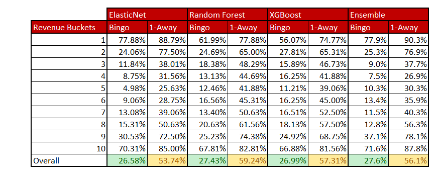
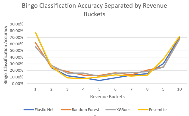
In our case, the Elastic Net Model performed best in the extreme revenue buckets (1,2,9,10) and the Random Forest model gives very good accuracy in the intermediate revenue buckets. This can be seen from the table displayed in the model comparison section.
###Rule Based Ensemble Approach Based on Class Level Accuracies###
data_movies$ensemble.predict<-ifelse(data_movies$el.predict %in% c(1,2,9,10), data_movies$el.predict, data_movies$rf.predict)
  ####Confusion matrix Creation###
  #table(data_movies$revenuebuckets, data_movies$xgb.predict)
  cm_ensemble<- as.matrix(table(Actual=data_movies$revenuebuckets,Predicted= data_movies$ensemble.predict))
  cm_ensemble
##       Predicted
## Actual   1   2   3   4   5   6   7   8   9  10
##     1  250  40   8   6   6   7   2   1   1   0
##     2  143  81  22  14  16  16   7   6  13   2
##     3  109  65  29  27  18  23  13   9  21   7
##     4   75  57  35  24  27  34  17  20  23   8
##     5   61  41  23  26  33  38  31  34  24  10
##     6   47  28  17  20  30  43  42  36  41  16
##     7   26  29  12  18  25  38  37  54  55  27
##     8   12  21   7  13  19  23  45  41  94  45
##     9   13   9   6   5  13  11  14  45 119  86
##     10   2   5   2   3   1   8   5  13  52 229
  cmdf_ensemble<- as.data.frame(cm_ensemble)
  cm_rs_ensemble<-reshape(cmdf_ensemble,idvar="Actual",timevar="Predicted", direction="wide")
  cm_rs_ensemble$Actual<-NULL
  rowsums = apply(cm_ensemble, 1, sum)
  cm_rs_ensemble$TotalActuals<- rowsums

  acc_fold_ensemble<-c()
  for (i in 1:nrow(cm_rs_ensemble))
    acc_fold_ensemble[i]<-cm_rs_ensemble[i,i]/cm_rs_ensemble[i,"TotalActuals"]
The bingo classification accuracy for the Ensemble Model is as follows,
final_acc_ensemble<- mean(acc_fold_ensemble)
final_acc_ensemble
## [1] 0.2764194
6. Model Comparison
The following figure shows the variation of bingo classification accuracy and 1-away classification accuracy across the revenue buckets as well as the overall accuracies.
We can observe how the classification accuracy is pretty high towards the extreme revenue buckets but it becomes extremely hard for the models to distinguish between the revenue buckets in the intermediate ranges as shown below.
The Random Forest model performs the best among the 3 traditional models that we have implemented with a Bingo Classification Accuracy of 27.43% and 1-Away Classification Accuracy of 59.24%.
7. Key Model Insights
1) Although several innovative features were used and had some relevance as seen in the Variable Importance Plot, the conventional variables like budget remained the primary factor driving movie box office success
2) In addition to directors and cast, the brand of the production company plays an extremely important role in how well a movie performs at the box office
3) The runtime of a film is one of the top 10 predictors affecting box office success
4) The network interaction scores have also features among some of the top 20 predictors to estimate movie box office success
8. Model Limitations
1) The movies dataset in Kaggle has not been through a thorough data quality analysis. There are many recent movies with incomplete revenues reported that we could have missed out in data cleaning process
2) The global revenues reported for each movie are not always consistently in US Dollars which necessitated filtering only English Language movies for our analysis
3) The movies dataset has a lot of text based features like movie overview, keywords etc. which can be explored using NLP techniques to further improve the model accuracy
9. Conclusion
The model comparisons show that Random Forest has proven to be the best statistical modelling method for this multinomial classification problem with a Bingo Classification Accuracy of 27.43% and a 1-Away Classification Accuracy of 59.43%. The Ensemble Model we built performed marginally better than our Random Forest Model on the Bingo Classification Accuracy measure. The primary research paper cited for the movie box office prediction was by Sharda which had a Neural Network Classifier perform the best with a Bingo Classification Accuracy of 36.9%. However the dataset used by the research paper was on a much smaller subset of our dataset(excluding a lot of old movies), had fewer revenue buckets and incorporated a lot of features from domain knowledge about the movie industry.
The performance of our models can be further enhanced by improving the completeness/reliability of revenue reported for the most recently released movies. There are other text based fields like keywords, movie overview which can be explored using NLP to improve model performance. However, the current features are a good starting point to improve on our prediction accuracy in the movie box office prediction problem.
10. References
1: Chuansun76. “Imdb-5000-movie-dataset.” Kaggle. N.p., n.d. Web. https://www.kaggle.com/deepmatrix/imdb-5000-movie-dataset
2: Sharda, Ramesh, and Dursun Delen. “Predicting Box-office Success of Motion Pictures with Neural Networks.” N.p., n.d. Web. http://citeseerx.ist.psu.edu/viewdoc/download?doi=10.1.1.85.679&rep=rep1&type=pdf
3: Im, Darin, and Minh Thao Nguyen. “PREDICTING BOX-OFFICE SUCCESS OF MOVIES IN THE U.S. MARKET.” PREDICTING BOX-OFFICE SUCCESS OF MOVIES IN THE U.S. MARKET (n.d.): n. pag. Http://cs229.stanford.edu. Web. http://cs229.stanford.edu/proj2011/ImNguyen- PredictingBoxOfficeSuccess.pdf
4: Merwe, Jason Van Der, and Bridge Eimon. “Http://cs229.stanford.edu/proj2013/vanderMerweEimon-MaximizingMovieProfit.pdf.” Predicting Movie Box Office Gross (n.d.): n. pag. Http://cs229.stanford.edu. Web. http://cs229.stanford.edu/proj2013/vanderMerweEimon-MaximizingMovieProfit.pdf
5: Arias, Marta. “Log-Linear Models and Logistic Regression.” Linear and Logistic Regression 40.3 (1998): 267-68. Www.cs.upc.edu. Fall 2012. Web.
6: Maji, Subhransu. “Binary Particle Classification.” Practical Guide to Machine Vision Software (2014): 191-208. Http://www.csee.umbc.edu. Web.
