
Time Series Forecasting - Part 2
Autoregressive-Integrated-Moving Average (ARIMA) modelling is another popular technique for time series forecasting which aims to describe autocorrelations in the data. While exponential smoothing methods do not make any assumptions about correlations between successive values of the time series, in some cases we can make a better predictive model by taking correlations in the data into account. Autoregressive Integrated Moving Average (ARIMA) models include an explicit statistical model for the irregular component of a time series, that allows for non-zero autocorrelations in the irregular component
Motivation
Prediction of the stock prices and precious metal prices is a widely studied subject by researchers. We attempt to leverage ARIMA modelling to forecast gold prices in this post.
Methodology
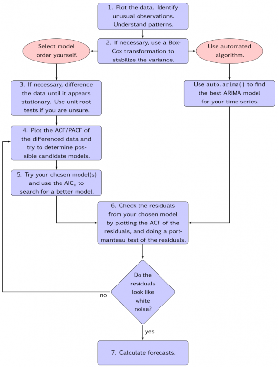
When fitting an ARIMA model to a set of time series data, the following procedure provides a useful general approach.
1) Visualize the data and identify any unusual observations.
2) If necessary, transform the data to stabilize the variance.
3) If the data are non-stationary: take first differences of the data until the data are stationary.
4) Examine the ACF/PACF: Is an AR(p) or MA(q) model appropriate?
5) Try the chosen models, and use the AIC metric to search for a better model.
6) Check the residuals from your chosen model by plotting the ACF of the residuals. If they do not look like white noise, try a modified model.
7) Once the residuals look like white noise, calculate forecasts.
The following process flow sourced from Rob Hyndman’s book on Forecasting provides a good overview of the steps involved in ARIMA modelling.
Data Overview
The dataset used for this problem has historical month over month gold prices from January, 1960 to December, 2017. We attempt to forecast the gold prices for the first 5 months in 2018.
The following code snippet includes the required packages in R for our analysis.
library(forecast)
library(fpp2)
library(ggplot2)
library(ggfortify)
library(forecast)
We can now take a quick look at a snapshot of our dataset.
tail(df_gold,5)
##       Month Price_per_Oz
## 692 2017M08      1283.04
## 693 2017M09      1314.07
## 694 2017M10      1279.51
## 695 2017M11      1281.90
## 696 2017M12      1264.45
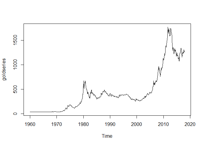
A quick visualisation of the gold prices since 1960 can be seen in the visualisation below,
goldseries <- ts(df_gold[,"Price_per_Oz"], start=c(1960,1),frequency=12)
plot.ts(goldseries)
Concept of Stationarity and Differencing
A stationary time series is one whose properties do not depend on the time at which the series is observed. So time series with trends, or with seasonality, are not stationary — the trend and seasonality will affect the value of the time series at different times. On the other hand, a white noise series is stationary — it does not matter when we observe it, it should look much the same at any period of time.
When building models to forecast time series data (like ARIMA), we start by differencing the data until we get to a point where the series is stationary. Models account for oscillations but not for trends, and therefore, accounting for trends by differencing allows us to use the models that account for oscillations.
From the visualization, we can see that the time series is not stationary and has an increasing trend over time. We can attempt to perform first differencing and then plot the resultant series to check if the series is stationary.
goldseries_diff <- diff(goldseries, differences=1)
plot.ts(goldseries_diff)
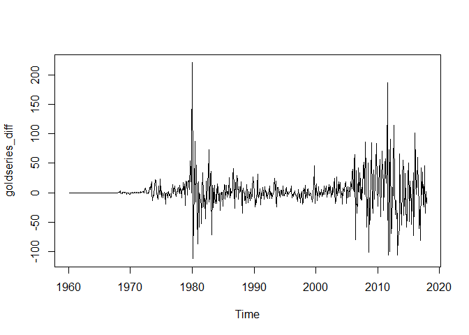
We can see that the resultant first differenced series is stationary. If it was not stationary with first differencing, we would attempt to perform higher order differencing to achieve stationarity.
Since the data is almost a horizontal line until 1980, we can use the data after 1980 only and recheck the first differencing plot.
df_goldfil <- tail(df_gold,-240)
goldseriesfil <- diff(df_goldfil[,"Price_per_Oz"], differences=1)
goldseriesfil_diff1 <- diff(goldseriesfil, differences=1)
plot.ts(goldseriesfil_diff1)

There is a very clear evidence of stationarity here. The first differenced series appears to be stationary with a constant mean and variance.
Selecting a candidate ARIMA Model
Let’s define the parameters of ARIMA(p,d,q) model that we will estimate:
p is the number of autoregressive terms, d is the number of nonseasonal differences, and q is the number of lagged forecast errors in the prediction equation. such that p, d, and q are integers greater than or equal to zero and refer to the order of the autoregressive, integrated, and moving average parts of the model, respectively. So p captures the order of an autoregressive model (a linear regression of the current value of the series against one or more prior values of the series); d is the order of the differencing used to make the time series stationary; and q is the order of the moving average model (a linear regression of the current value of the series against the white noise or random shocks of one or more prior values of the series).
If the time series is stationary, or if we have transformed it to a stationary time series by differencing d times, the next step is to select the appropriate ARIMA model, which means finding the values of most appropriate values of p and q for an ARIMA(p,d,q) model. To do this, we usually need to examine the correlogram and partial correlogram of the time series.
To plot a correlogram and partial correlogram, we can use the “acf()” and “pacf()” functions in R.
acf(goldseriesfil_diff1,lag.max=20,main="AutoCorrelogram")
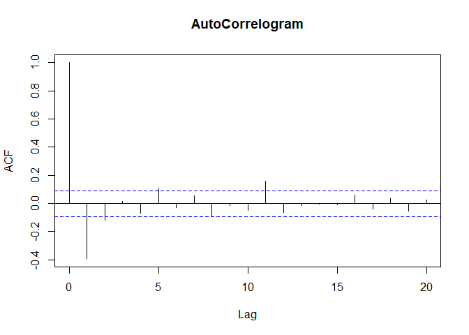
pacf(goldseriesfil_diff1,lag.max=20,main="Partial AutoCorrelogram")
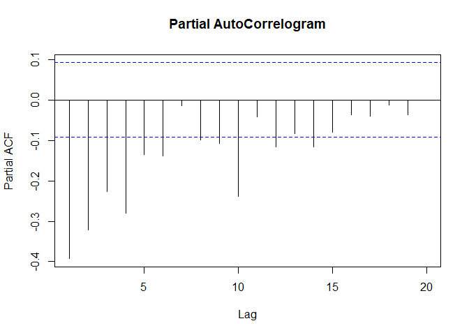
The autocorrelogram shows that the autocorrelations for 2 lags exceed the significant bounds comprehensively. The partial auto correlogram looks like it is dying out slowly. The possible candidate models from the ACF and PACF plots are,
- ARMA(0,3)
- ARMA(1,2)
- ARMA(2,1)
In the manual process, we can compare each of these candidate models based on their AIC to obtain the final values of p and q.
ARIMA using auto.arima()
In R, as seen in the process flow above, we can use the auto.arima() function to skip the previous manual selection process involved in identifying the p,d,q values.
goldseries_arima <- auto.arima(goldseries)
goldseries_arima
## Series: goldseries
## ARIMA(1,1,2) with drift
##
## Coefficients:
##           ar1     ma1     ma2   drift
##       -0.7603  0.9654  0.1002  1.7552
## s.e.   0.1119  0.1207  0.0574  1.1353
##
## sigma^2 estimated as 654.6:  log likelihood=-3237.41
## AIC=6484.82   AICc=6484.9   BIC=6507.54
We can see that the auto.arima() model picks the best values of p,d,q to be 1,1,2. It first differences the non stationary series and on the stationary series it picks an ARMA(1,2) model to be the best fit.
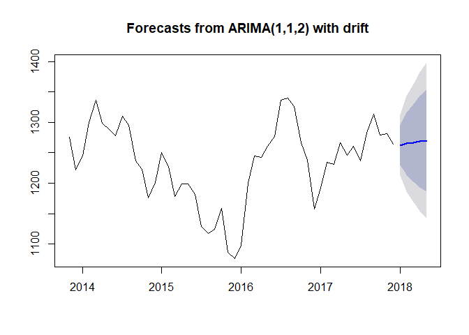
With the model suggested by auto.arima() we can make forecasts for 5 subsequent months in 2018 and plot it using the forecast function in R.
goldseries_forecasts <- forecast(goldseries_arima, h=5)
plot(goldseries_forecasts, include = 50)
Similar to the test for model quality in Holt-Winters method, we check for the quality of forecasts in ARIMA by investigating the forecast errors. We investigate whether the forecast errors seem to be correlated, and whether they are normally distributed with mean zero and constant variance. To check for correlations between successive forecast errors, we can make a correlogram and use the Ljung-Box test:
acf(goldseries_forecasts$residuals,lag.max=20,main="Residuals Autocorrelation")
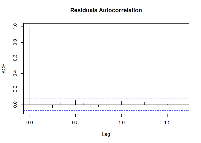
Box.test(goldseries_forecasts$residuals, lag=20, type="Ljung-Box")
##
## 	Box-Ljung test
##
## data:  goldseries_forecasts$residuals
## X-squared = 29.21, df = 20, p-value = 0.08371
The p-value of the Ljung-Box test is 0.083 indicating that there is very little evidence of autocorrelation in residuals. This can be confirmed from the autocorrelation plot of the residuals that we have plotted.
We can now test whether the forecast errors are normally distributed with mean zero and constant variance.
plot.ts(goldseries_forecasts$residuals)
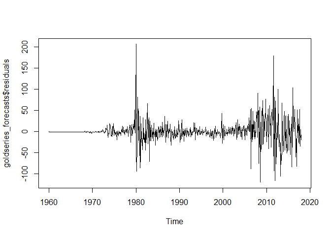
plotForecastErrors(goldseries_forecasts$residuals)

The plots indicate that the forecast errors have a mean very close to zero(~0.0073) and a constant variance. The model has passed the quality tests and the ARIMA(1,1,2) model that we have identified provides robust forecasts.