Time Series Forecasting - Part 1

Forecasting techniques have a range of applications such as stocking inventory in warehouses, scheduling staff in call centers, generating electricity in power plants etc. Forecasting has always been an effective aid for efficient planning. The predictability of an event depends on answers to 3 questions :

1) How well we understand the factors that contribute to it

2) How much data is available

3) Whether the forecasts can affect the event we are trying to forecast

When an event to be predicted meets all three basic conditions, the forecasts tend to be highly accurate. On the contrary, when one or more of the conditions are not met, the forecasts could just be as good as flipping a coin. In forecasting, a key step is understanding these factors associated with the event. Good forecasts capture the genuine patterns and relationships which exist in the historical data, but do not replicate past events that will not occur again.

If there is no data available, or if the data available is not relevant to the forecasts, then qualitative forecasting methods must be used. Quantitative forecasting on the other hand can be applied when two conditions are satisfied:

1) Numerical information about the past is available;

2) It is reasonable to assume that some aspects of the past patterns will continue into the future.

Most quantitative forecasting problems use either time series data (collected at regular intervals over time) or cross-sectional data (collected at a single point in time).

Two primary methods that are widely used for quantitative forecasting using univariate time series data are,

1) Exponential smoothing

2) Autoregressive Integrated Moving Average(ARIMA) model

These univariate time series forecasting methods are used especially when we do not capture other covariates that affect the event and we know that future occurrences of the event can be estimated from historical observations of the event.

In this post, we will explore one class of univariate forecasting methods - Exponential smoothing.

Problem Motivation

Forecasts based on temperature is important to agriculture, and therefore to traders within commodity markets. They are used by utility companies to estimate future demand for utilities. Our main motivation behind this exercise is to present a feasible time series model to forecast the weekly average temperature in Austin, Texas.

Data Overview

The dataset for the problem is sourced from Kaggle and contains historical temperature for Austin, Texas. The dataset has information at a daily grain from December 21, 2013 to July 31, 2017.

Since the dataset shows daily volatile fluctuations, the time series is aggregated at a weekly grain to better capture the weather pattern. Of the 187 weeks, we use data from 182 weeks for estimating the model. Out of sample forecasts are then made from week 183 to week 187 using the estimated model parameters. The actual values can then be compared to the forecasted values to test the model fit.

The following code snippet includes the required packages in R for our analysis.

library(forecast)
library(fpp2)
library(ggplot2)
library(ggfortify)
library(forecast)

We can take a quick look at a snapshot of our dataset.

head(df_train,5)

##   Week Temp_Avg
## 1    1    47.29
## 2    2    51.00
## 3    3    55.57
## 4    4    50.29
## 5    5    49.29

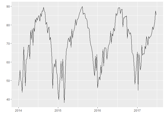
The following snippet takes the time series data frame, name of the feature to be estimated, frequency of data collection and start time as inputs to generate a visualization of the time series.

plot_my_timeseries<- function(df_select,featurename,frequency,start_ym)
{
  arg_df<- df_select[,featurename]
  start_date <- start_ym
  freq <- frequency ####12 for Monthly, 52 for weekly, 365 for daily and so on
  timeseries_obj <- ts(arg_df,start=start_date,frequency=freq)
  autoplot(timeseries_obj)
}

plot_my_timeseries(df_train,c("Temp_Avg"),52,c(2014,1))

Forecasting Techniques

Exponential Smoothing and ARIMA models are the two most widely-used approaches in univariate time series forecasting, and provide complementary approaches to the forecasting problem. While exponential smoothing models are based on a description of trend and seasonality in the data, ARIMA models aim to describe autocorrelations in the data. Let us first explore the Holt-Winters Exponential Smoothing method.

Holt-Winters Exponential Smoothing

The Holt-Winters model has a forecast equation and 3 smoothing equations to estimate the time series. Firstly, the level (or mean) is smoothed to give a local average value for the series. Secondly, the trend is smoothed and lastly each seasonal sub-series is smoothed separately to give a seasonal estimate for each of the seasons. The 3 smoothing parameters estimated are - alpha for level, beta for trend and gamma for seasonality.

There are two variations to this method that differ in the nature of the seasonal component. The additive method is preferred when the seasonal variations are roughly constant through the series, while the multiplicative method is preferred when the seasonal variations are changing proportional to the level of the series. We will explore the additive variation of the method since our seasonal variations are roughly constant throughout the series as seen from our visualization.

The parameters alpha, beta and gamma all have values between 0 and 1, and values that are close to 0 mean that relatively little weight is placed on the most recent observations when making forecasts of future values.

We use the HoltWinters() function in R to make forecasts using this method.

ts_hw <- ts(df_train[,"Temp_Avg"],start=c(2014),frequency=52)
hw_model <- HoltWinters(ts_hw)
hw_model$alpha

##       alpha
## 0.002523082

hw_model$beta

##      beta
## 0.1347367

hw_model$gamma

##     gamma
## 0.7946229

The estimated values of alpha, beta and gamma are 0.002, 0.134, and 0.794, respectively. The value of alpha is relatively low, indicating that the estimate of the level at the current time point is based on some observations in the more distant past. The value of beta is low at 0.134, indicating that the estimate of the slope of the trend component is not updated over the time series. Intuitively this makes sense, as the level changes quite a bit over the time series, but the slope of the trend component remains roughly the same. The value of gamma is high, indicating that the estimate of the seasonal component at the current time point is just based upon very recent observations.

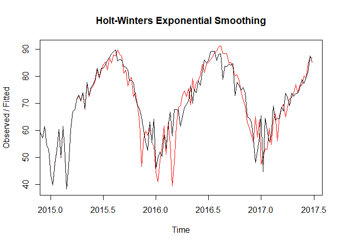
In the plot given below we compare the original time series(in black) with the in-sample forecasts from the Holt-Winters method(in red). We notice from the plot that the Holt-Winters method captures the seasonal peaks very well.

We can make forecasts for further time points by using the “forecast” function in the R “forecast” package. When using the forecast() function, we pass the predictive model that we have already fitted using the HoltWinters() function. We can also specify how many further time points we want to forecast for using the “h” parameter. We take h=5 as we want to make predictions for 5 subsequent weeks. The out of sample forecasts from the Holt-Winters model can be seen below.

hw_forecasts <- forecast(hw_model, h=5)
plot(hw_forecasts)

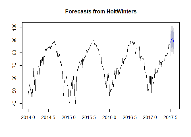
The point forecasts are shown as a blue line, and the 2 bands show 80% and 95% prediction intervals, respectively. The prediction intervals are important as they represent the uncertainty associated with the point forecast.

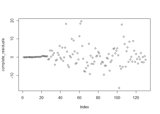
We now test the quality of our Holt-Winters model. This is done by checking if the in-sample forecast errors have a constant variance over time, and are normally distributed with mean zero.

residuals <- hw_forecasts$residuals
complete_residuals <- residuals[complete.cases(residuals)]
plotForecastErrors <- function(forecasterrors)
{
  # make a histogram of the forecast errors:
  mybinsize <- IQR(forecasterrors)/4
  mysd   <- sd(forecasterrors)
  mymin  <- min(forecasterrors) - mysd*5
  mymax  <- max(forecasterrors) + mysd*3
  # generate normally distributed data with mean 0 and standard deviation mysd
  mynorm <- rnorm(10000, mean=0, sd=mysd)
  mymin2 <- min(mynorm)
  mymax2 <- max(mynorm)
  if (mymin2 < mymin) { mymin <- mymin2 }
  if (mymax2 > mymax) { mymax <- mymax2 }
  # make a red histogram of the forecast errors, with the normally distributed data overlaid:
  mybins <- seq(mymin, mymax, mybinsize)
  hist(forecasterrors, col="red", freq=FALSE, breaks=mybins)
  # freq=FALSE ensures the area under the histogram = 1
  # generate normally distributed data with mean 0 and standard deviation mysd
  myhist <- hist(mynorm, plot=FALSE, breaks=mybins)
  # plot the normal curve as a blue line on top of the histogram of forecast errors:
  points(myhist$mids, myhist$density, type="l", col="blue", lwd=2)
}
plot(complete_residuals) # constant variance over time

plotForecastErrors(complete_residuals) # make a histogram to check distribution of forecast errors

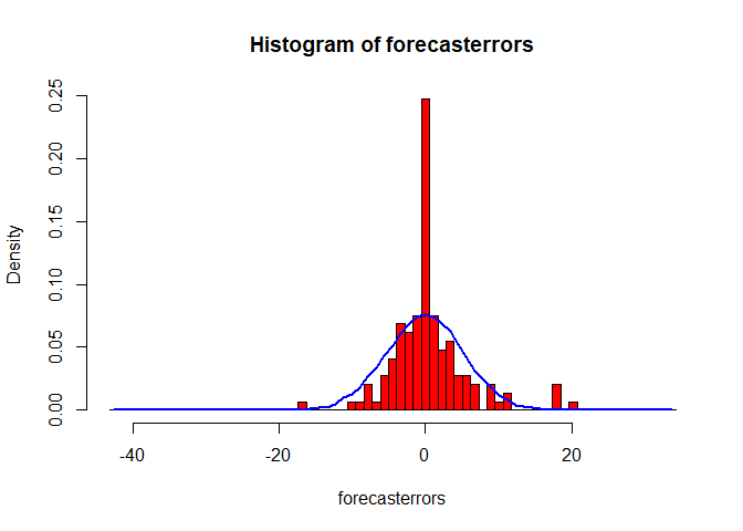
From the above plots, we notice that the forecast errors have a constant variance over time and they are normally distributed with mean zero. This verifies the assumptions based on which prediction intervals are estimated.

We further test the model quality by measuring the out of sample performance using the evaluation metric Mean Average Percentage Error(MAPE).

###Compare forecasts with actual test###
df_test <- df_weather[df_weather$split=="TEST",c("Week","Temp_Avg")]
actuals_test <- df_test$Temp_Avg
forecasts_test <- as.numeric(hw_forecasts$mean)
MAPE = mean(abs((actuals_test-forecasts_test)/actuals_test))
MAPE

## [1] 0.02396997

A MAPE of 2.4% indicates that the model performs well out of sample as well. We will explore the Autoregressive Integrated Moving Average model for univariate forecasting in a subsequent post.